How to build a Loss Exceedance Curve

In a Google Sheet

Image Generated by Gemini

This explainer document shows how to build a simple, first draft, Loss Exceedance Curve using common spreadsheet software (Google Sheets) and following the methodology outlined in Hubbard & Seiersen’s book, “How to Measure Anything in Cybersecurity Risk,” the techniques described in Tetlock and Gardner’s book, “Superforecasting,” the ballpark approximations made famous by Dr. Enrico Fermi, the forecasting power of Bayes’ Algorithm, and the methodologies detailed in my Cybersecurity First Principles book.

To demonstrate, I will use Perplexity.AI as a sample organization with an annual revenue of $20 million.

Note: You can follow along using the Google document: “Perplexity.AI Risk Forecasting Spreadsheet.”

Background: The Cybersecurity First Principle

From my “Cybersecurity First Principles” book, I made the case for the absolute cybersecurity first principle that applies to all organizations regardless of their size or vertical:

Reduce the probability of material impact due to a cyber event in the next business cycle.

If that’s accurate, information security professionals must understand the organization’s current risk level in order to demonstrate any reductions to senior leadership. Although Heat Maps are widely used to visualize risk for leadership audiences, repeated research shows that Heat Maps are scientifically flawed and unsuitable for this purpose. Instead, many leading risk experts, including Hubbard and Seiersen, recommend using the Loss Exceedance Curve.

Loss Exceedance Curves

A Loss Exceedance Curve is a visualization tool that demonstrates probability-of-loss estimates for certain cost thresholds within a specified time period. For our Perplexity.AI Loss Exceedance Curve, we are charting the probability of material loss within the next year. When we are done, it will look something like this example from the Hubbard and Seiersen book:

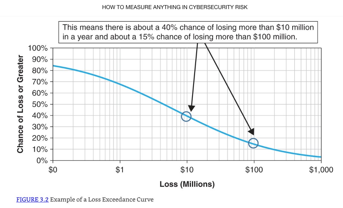
Risk forecasters generate the curve data (the blue line) using Monte Carlo Simulations.

Monte Carlo Simulations

A Monte Carlo Simulation is a computational technique that allows the forecaster to consider the likelihood of a range of potential outcomes. It is a mathematical model that represents a real world event we are trying to forecast. In our case, we are trying to model the estimated dollar loss of a Perplexity.AI cyber event.

A model can be simple, quite complex, or anything in the middle. Hubbard & Seiersen’s book covers the spectrum. For this Perplexity.AI example, we are using the first model they discuss in their book. I think it’s the most straightforward.

When we run the model one time, we get one output of an estimated dollar loss. When we run it a second time, we will get a different value. When we run it 10,000 times, we will have a collection of dollar loss values that range from the small to the big relatively.

To build the Loss Exceedance Curve, we are interested in the dollar loss due to a cyber event at various levels. How often does the dollar loss exceed $100K, $500K, $1M, etc? With a Monte Carlo Simulation, the forecaster runs the model thousands of times, collects the range of answers, and displays the frequency in bands of occurrence. Here is a simplified example:

• 10%: Less than $100K

• 30%: Between $100K and $500K

• 40%: Between $500K and $1M

• 20%: Greater than $1M

The last enhancement to the Hubbard & Seiersen model is to also account for the Perplexity.AI’s known probability of a cyber event. I’m going to show how to calculate that number below, but for this example, let’s say it's 20%. When we run the Monte Carlo Simulation thousands of times, we will only collect the dollar loss for our frequency array if a generated random number is below 20%.

You may or may not like Hubbard & Seiersen’s construct. If you don’t, you are probably already thinking about ways you might model it differently. That’s perfectly fine. Like I said, check out their book for more complex models. But, these kinds of simulations are valuable for simulating complex systems where the relationships between variables are not straightforward and/or the data for precise measurement isn’t generally available. Like I said, they are models. As the British statistician George E. P. Box said, “All models are wrong, but some are useful.” I say that this simple model is useful enough to inform our resource decisions.

Calculating Perplexity.AI’s Probability of a Cyber Event: Outside-In, then Inside-Out

For all loss exceedance curves, we start by making an Outside-In assessment. Outside-In is the generic case. What is the probability that any organization similar to Perplexity.AI, in terms of size and revenue, will experience a material cyber event in the next year. It’s Outside-In because we are not looking at Perplexity.AI specifically. We are just looking at public data for the entire population of companies like Perplexity.AI without any regard to how strong or weak their individual infosec programs are. In effect, we are counting the number of Perplexity.AI-like cyber victims compared to the entire population of Perplexity.AI-like companies and calculating a percentage.

According to the Superforecaster book, this percentage isn’t accurate or precise yet, but it’s in the right ballpark in terms of orders of magnitude of what the “true” answer is. In line with Bayes’ Algorithm, this is our first estimate. The next step is to collect more evidence.

We do that by conducting an Inside-Out analysis. What is our risk reduction estimate when considering our deployed cybersecurity strategies and tactics? For example, if Perplexity.AI has a mature deployment of its Zero Trust strategy, we would adjust the Outside-In forecast down by some amount. This would be our new cyber event forecast.

Continuous Probability Distributions

Risk forecasters use Continuous Probability Distributions to model random variable values with a Probability Density Function (PDF). For our purposes, the PDF will be a spreadsheet math formula that describes the likelihood of our model’s variables taking on specific values within a given range. After running the model ten thousand times, the answers outline the distribution’s shape.

Arguably, the most well known distribution shape is the Bell Curve (Normal Distribution) where the PDF generates data points that cluster around the mean and the frequencies of values decrease as they move away from the mean in either direction. But for our purposes, the Bell Curve is not the right shape.

Wide-enough distributions designed to capture some extreme events could produce illogical negative numbers on one the left of the scale (you can't have a negative dollar value lost for example). Per Hubbard and Seiersen’s book, we will use the Lognormal distribution instead. Those PDFs can't generate negative dollar values on the left side of the scale but can generate extreme dollar values on the right side. In the forecasting business, experts call this a long tail.

The reason this is important to distinguish is because modern day spreadsheets have built-in functions that produce different distributions. We’re going to use them.

Step by Step Instructions to make an Perplexity.AI Loss Exceedance Curve

Reminder: You can follow along with this example in this Google Sheets spreadsheet.

In order to build a Monte Carlo Simulation where we estimate the probability of material loss due to a cyber event, we create a Sheets formula for one run of the model, collect the data, and then run the model 10K times capturing the results each time. In Sheets, we will use the following functions:

• if()

• rand()

• ln()

• lognorm.inv()

The if() Function

Used to make decisions in your spreadsheet by testing if a condition is true or false, and then returning a different result based on that check.

=if(logical_expression, value_if_true, value_if_false)

=if(.2 < 0.8,1,0)

will return a 1 because it is true.

The rand() Function

Generates a random decimal number between 0 and 1 (not including 0 and 1 themselves). Every time the spreadsheet updates or recalculates, it produces a new random number.

=if(rand() < 0.8,1,0)

In this example, if the generated random number is less than 80%, the function returns a 1. If it's greater, it returns 0 (See Google Sheets spreadsheet Tab: “From the Book”)

To generate another random number, you have to force Sheets to recalculate. There are many ways to do this in Sheets but the way I did it was by creating a checkbox.

From the Menu on the top left of the spreadsheet

Insert

Checkbox

Every time you click the Checkbox, Sheets recalculates another random number.

The ln() Function

Calculates the natural logarithm of a number. Since we are using a Lognormal distribution, we need to keep all the numbers in that form.

The natural logarithm is a special type of logarithm with a base called Euler's number, approximately 2.718. This function tells you what power you need to raise this base (e) to get the number you're interested in. For example, if you use =ln(10), it will give you around 2.303 because e raised to the 2.303 power is about 10. It only works for positive numbers greater than zero. If you try to use zero or a negative number, you get an error.

=ln(value)

The lognorm.inv() Function

Answers questions like, what’s the highest value I’d expect to see with a certain level of probability?

x = lognorm.inv (probability, mean, standard_dev)

If you know the probability, the mean and standard deviation of ln(data), this function tells you the real-world value associated with that chance. Said differently, for a given chance, what’s the biggest dollar loss likely to occur?” We are going to use it for our Probability Density Function (PDF) to calculate dollar loss scenarios.

Normally, risk forecasters calculate the mean and the standard deviation based on the width of the probability distribution. According to Hubbard & Seiersen though, most people who don’t do stats for a living find the concept non-intuitive. Instead, based on their recommendation, we will use a 95% Confidence Interval (CI) based on an upper bound (UB) and lower bound (LB) of potential losses provided by an expert. The expert in our case is the 2024 IRIS Ransomware report by Cyentia. Specifically, we want to look at “Table 1: Loss statistics by revenue tier” on page 16.

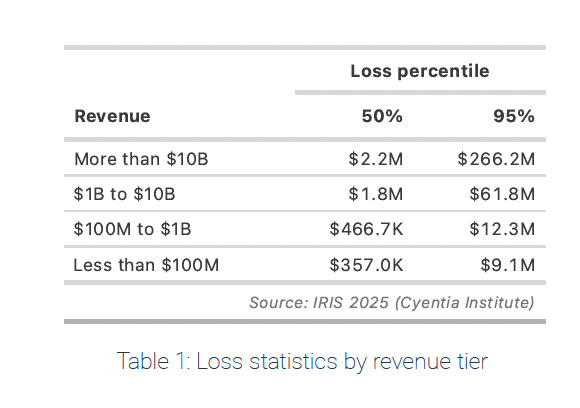
As of April 2025, analysts at TapTwice Digital estimate that Perplexity.AI generates approximately $20 million in annual revenue. According to the Cyentia table then, the upper bound is $9.1M and the lower bound is $375K.

Since we are using the The lognorm.inv() function though, we have to use the natural logarithm of a number. For the mean, we will use

ln($9.1M) + ln($375K)) / 2

which is the distance between the Upper Bound and Lower Bound divided by 2.

For the standard deviation, we will use the Hubbard and Seiersen standard deviation estimate formula: log of the Upper Bound - the log of the Lower Bound divided by 3.29.

ln($9.1M) - ln($375K)) / 3.29

Hubbard and Seiersen use the constant 3.29 because, in a log-normal distribution, the range from the 5th percentile to the 95th percentile is approximately 3.29 standard deviations wide. This estimation assumes that the range from Upper Bound to Lower Bound covers approximately 90% of the data.

For our Perplexity.AI PDF, we now have a way to calculate the mean and the standard deviation. For the probability variable, we will use the rand() function again to generate random dollar loss values for each run of the simulation.

x=if (rand() <0.063, lognorm.inv (rand(), (ln($9.1m) + ln($325k)) / 2, (ln($9.1M) - ln($325k)) / 3.29), 0)

Probability of a Perplixity.AI Cyber Event

Each time we run the simulation, we want to make sure that the occurrence frequency matches Perplexity.AI’s estimated probability of a cyber event within the next year. Our PDF should look like this:

x=if (rand() < probability of a cyber event, lognorm.inv (rand(), ln($9.1M) + ln($375K)) / 2, ln($9.1M) - ln($375K)) / 3.29), 0)

If a random percentage is less than the estimated probability, then we record that dollar loss. If it’s greater, then we don’t.

But how do we determine what the probability of a cyber event is? We go back to the Cyentia experts.

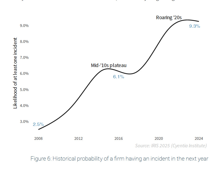
From “Figure 6: Historical probability of a firm having an incident in the next year” of the same Cyentia 2024 IRIS Ransomware report, the Outside-In probability that a typical firm, not just Perplexity.AI but all firms, will experience a cyber event is about 9.3%. That’s the general case for all organizations. But, if we assume that Perplexity.AI has deployed a zero trust strategy that, after our Inside-Out analysis, reduces the probability of a cyber event by another 3%, then, doing the math (9.3% - 3%), the probability of a Perplexity.AI cyber event in the next year is 6.3%. Our PDF then, will look like this:

x=if (rand() <0.063, lognorm.inv (rand(), ln($9.1M) + ln($375K)) / 2, ln($9.1M) - ln($375K)) / 3.29), 0)

To run the Monte Carlo simulation 10,000 times

• Make two columns in a Sheets Spreadsheet: Simulation Number and Loss Value.

• Make a Checkbox (as described above)

• In the Simulation Number column, countdown from 1 - 10,000.

• In the Loss Value column, copy the Monte Carlo Simulation PDF into each cell adjacent to the Simulation Number.

• Make a new Sheets tab (“Just the Data”)

  • from the bottom left of the spreadsheet, Click the "+" button

  • Right Click the new tab

  • Rename the new tab to "Just the Data"

• Copy just the Monte Carlo values from all 10,000 cells to the "Just the Data" tab

  • Highlight the Two Columns

  • Edit

  • Copy

• Move to the "Just the Data" tab

  • Edit

  • Paste Special

  • Values Only

Create a Loss Exceedance Curve histogram

In the "Just the Data" tab, create three more columns: Cost, Percentage, and Count.

Under the "Cost" column, make nine rows with the following text:

"No Cost

> $1K

> $10K

> $100K

> $1M

> $10M

> $100M

> $1B

> $10B

For the "Count" column, we want to count how many times the values in the "10,000 simulations" fall into each of these categories.

In Sheets, we use the countif() function to look for one condition

=countif(B4:B10007,"=0")

We use the countifs() function to look for multiple conditions

=COUNTIFS(B4:B10007, ">0", B4:B10007, "<10000")

For the cells adjacent to the "Cost" rows, add the formula

No Cost: =countif(B2:B10005,"=0")

< $1K: =countif(B2:B10005,">1000")

< $10K: =countif(B2:B10005,">10000")

> $100K: =countif(B2:B10005,">100000")

> $1M: =countif(B2:B10005,">1000000")

> $10M: =countif(B2:B10005,">10000000")

> $100M: =countif(B2:B10005,">100000000")

> $1B: =countif(B2:B10005,">1000000000")

> $10B: =countif(B2:B10005,">10000000000")

For the Percentage Column, we want to turn the values in the "Cost" column into a percentage by dividing each by 10,000 (The number of Monte Carlo samples):

=G20/10000

Create the Loss Exceedance Curve

• Highlight the column titles and data for "Cost" and "Percentage"

• Use Sheets to build the Chart

  • Top Left Menu

    • Insert

    • Chart

  • Top Right Chart Editor Menu

    • Setup

    • Chart Type

    • Line Chart

    • Customize

    • Chart Style

    • Check: Smooth

    • Chart Axis and Titles

    • Title text: Perplexity.AI Risk Forecast for September 2025 to September 2026

    • Title Format: Center

    • Series

    • Check: Data Labels

    • Gridlines and Ticks

    • Check: Major Gridlines

    • Check: Minor Gridlines

    • Check: Major Ticks

    • Check: Minor Ticks

    • Check: Vertical Axis : log scale

and this is what you get

Material Cyber Risk vs Cyber Risk

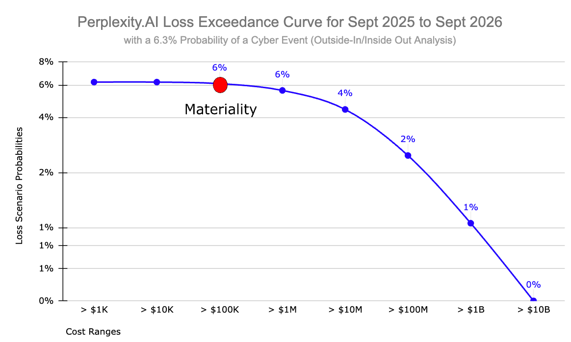
Look closely at the subtitle of that Loss Exceedance Curve: “with a 6.3% Probability of a Cyber Event (Outside-In/Inside-Out Analysis).” It shows you the probability that Perplexity.AI will experience some kind of cyber event within the next year that will cost the company anywhere from $1K to $1B. The chances are remarkably small ranging from 6% for a 10K loss to 1% for $1B loss. But still, there’s a chance. Even so, a cyber event is not a material cyber event.

As I said at the top of this essay, I believe that the absolute cybersecurity first principle is to reduce the probability of “material” impact due to a cyber event in the next business cycle. A cyber event that costs the company $10K is painful, but it might not be material to the business.

And I hear what you’re probably saying to yourself. “So, what does material mean then?” That’s a good question. Let me just say that the answer is complicated and depends on the culture of the company and the risk tolerance of the senior leadership team and the board. Every organization is different. Entire books have been written about the subject. For the purposes of this discussion though, let’s use a standard practice. One CPA Test firm that I found says that a common starting point for materiality in a $20 million revenue company is about 1% of revenue (around $200,000). That’s good enough for what we are trying to do here. I put a red dot on the cost line to show where that number falls on the Loss Exceedance Curve.

That means that, for Perplexity.AI, the probability of a material cyber event in the next year is about 6%.

Take Away

I’ve been studying cyber risk forecasting techniques for about ten years now. Research shows that Qualitative Heat Maps are a bad way to convey risk to senior leadership. The better way is to use Loss Exceedance Curves to to demonstrate probability-of-loss estimates for certain cost thresholds within a specified time period.

But, the average infosec practitioner couldn’t easily build them unless they were a statistics nerd and just liked that kind of thing. The process is filled with all kinds of new and scary terms like Monte Carlo Simulations, Continuous Probability Distributions, Probability Density Functions, and Lognormal Distributions. But, it turns out that, once you get the general meaning of what all those things are, they reduce to just fancy math terms that can easily be leveraged using common desktop software like Google Sheets. All you need are five variables:

1. Upper and Lower Bound

2. Outside-In Probability of a Cyber Event

3. Inside-Out Probability of a Cyber Event

4. Probability of a Cyber Event

5. Material Dollar Loss Amount

This is not rocket science. With a nod to Dr. Enrico Fermi, the use of a Loss Exceedance Curves is just a back-of-the-envelope visualization tool that will allow security professionals to inform important resource decisions.

For Perplexity.AI, we now know that they have a roughly 6% chance of experiencing a material cyber event within the next year. With that information, infosec professionals and senior leadership can evaluate their organization’s risk tolerance and decide what they want to do about it. If they are fine with the 6% risk, then nothing much has to change. If they would like that percentage to be smaller, then there are first principle strategies to consider that might do that. But that is a different discussion.

References

Bryan Smith, 2019. How to Read Loss Exceedance Curves in RiskLens [Explainer]. RiskLens. URL https://www.risklens.com/resource-center/blog/reading-loss-exceedance-curves

Douglas Hubbard, Richard Seiersen, 2016. How to Measure Anything in Cybersecurity Risk [Book]. Goodreads. URL https://www.goodreads.com/book/show/26518108-how-to-measure-anything-in-cybersecurity-risk

Guillem Barroso, 2018. George Box Quote: “All models are wrong, but some are useful” [Explainer]. AdMoRe. URL https://www.lacan.upc.edu/admoreWeb/2018/05/all-models-are-wrong-but-some-are-useful-george-e-p-box/

Philip Tetlock, Dan Gardner, 2015. Superforecasting: The Art and Science of Prediction [Book]. Goodreads. URL https://www.goodreads.com/book/show/23995360-superforecasting

Rick Howard, 2023. Cybersecurity First Principles: A Reboot of Strategy and Tactics [WWW Document]. Amazon. URL https://www.amazon.com/Cybersecurity-First-Principles-Strategy-Tactics-ebook/dp/B0C35HQFC3/ref=sr_1_1

Rick Howard, August 29 2025. Perplexity.AI Risk Forecasting Spreadsheet [Spreadsheet] First Principles Consulting. URL: https://docs.google.com/spreadsheets/d/1eXI3uZzvrQUmyfZXGKBJF1HS5g-DF8NYAuJFJMiZH2s/edit

Rick Howard, 2025. Heat Maps are Just Bad Science [Explainer]. Rick’s First Principles Newsletter - Substack. URL https://diffuser.substack.com/p/heat-maps-are-just-bad-science

Sharon Bertsch McGrayne, 2011. The Theory That Would Not Die: How Bayes’ Rule Cracked the Enigma Code, Hunted Down Russian Submarines, and Emerged Triumphant from Two Centuries of Controversy [Book]. Goodreads. URL https://www.goodreads.com/book/show/10672848-the-theory-that-would-not-die

Staff, 2021. Fermi Problem Explained [Video]. Inch by Inch Stories. URL

Staff, 2024. IRIS Ransomware [Analysis]. Cyentia Institute | Data-Driven Cybersecurity Research. URL https://www.cyentia.com/iris-ransomware/

Staff, 2025. AUD CPA Exam: How to Calculate Materiality for an Entity’s Financial Statements as a Whole [Explainer]. SuperfastCPA CPA Review: URL https://www.superfastcpa.com/aud-cpa-exam-how-to-calculate-materiality-for-an-entitys-financial-statements-as-a-whole/

Staff, 2025. 7 Perplexity AI Statistics (2025): Revenue, Valuation, Investors, Funding [Analysis]. TapTwice Digital. URL https://taptwicedigital.com/stats/perplexity.

Staff, n.d. What Is Monte Carlo Simulation? [Explainer]. IBM. URL https://www.ibm.com/topics/monte-carlo-simulation